Download links:
My full framework is available for free on the Matlab File Exchange:
http://www.mathworks.com/matlabcentral/fileexchange/51120-parallel-particle-swarm-optimizer-for-cuda-c-models
Summary:
For this project, I created a Matlab/Cuda framework that allows users to easily
implement, optimize and visualize their CUDA/C models. The framework has two components:
First is a GPU-parallelized particle swarm optimizer in Matlab that allows full utilization of GPU hardware for faster optimization using a research-verified particle swarm variant (1). The optimizer also allows the user to test all different types of launch bounds straight from Matlab for easy profiling and meta optimization.
The second part is a mex file that contains a wrapper kernel with the cuRand random number generation and data reduction routines already in place. It also contains a main function with all the mex-specific-code and gpu error checking routines in place. This allows easy integration with the users' specific model and fast debugging.
Lastly, I include a demonstration of this framework by showing the results of running the particle swarm optimizer on my own CUDA/C MCMC model that predicts the behavior cardiac muscle tissue. I will also demonstrate how to use my framework for profiling/meta optimization.
The resulting framework can easily be adapted to multi GPU solutions or other optimization techniques that can be paralleled across generation.
Background:
Particle swarm optimization has a big sequential limitation: All particles must be updated generation by generation. However, there lies a huge potential for parallelization across all particles in a particular generation. Let's take a look at the serial PSO.
In a serial PSO, there are several particles that explore a search space, looking for the optimal parameters in terms of lowest associated "cost" in a user-specified objective function. This cost is just a scalar value that the user is trying to minimize.
Each particle is represented by a single parameter set that evolves over iterations in response to two things:
1) the "cost" associated with those particular parameters when evaluated in the objective function.
2) the "cost" associated with the particle that yielded the lowest cost thus far across all particles in the swarm (global best).
In its most basic form, each particle will initialize itself to random positions and velocities and evolve according to the following equation where C1 is a constant representing how heavily to weigh the global best particle in the next position shift. C2 is a constant representing how heavily to weigh the particle's own personal best in the next position shift:
 for all PSO iterations:
for each particle, p:
cost = calculate fitness(p.current_position)
if cost < global_best_cost:
global_best = p.current_position;
global_best_cost = cost;
if cost < p.personal_best_cost:
p.personal_best = p;
p.personal_best_cost = cost;
p.velocity = p.velocity +
C1 * (global_best - p.current_position ) +
C2 * (p.personal_best - p.current_position)
p.current_position= p.current_position +
p.velocity
for all PSO iterations:
for each particle, p:
cost = calculate fitness(p.current_position)
if cost < global_best_cost:
global_best = p.current_position;
global_best_cost = cost;
if cost < p.personal_best_cost:
p.personal_best = p;
p.personal_best_cost = cost;
p.velocity = p.velocity +
C1 * (global_best - p.current_position ) +
C2 * (p.personal_best - p.current_position)
p.current_position= p.current_position +
p.velocity
Essentially, particles evolve and converge over time to the particle that has found the lowest cost thus far while being biased to the coordinates associated with their own personal-lowest cost.
For my project, I parallelized this algorithm across particles in one PSO iteration. The Matlab file calls the mex file containing a framework I built to easily utilize cuRand and reduce data in parallel. The mex file takes batch size as an argument to create an appropriate number of CUDA streams which run individual particles simultaneously. Particles are encoded as a single array of concatenated particle positions. The main arguments that the PSO takes are the number of threads, thread blocks, batch size, and search space bounds to run the model with. Other arguments tune the PSO and are already set to values that have been validated by research on PSOs.
The key data structures are four matrices in the Matlab parallel PSO code which encode current particle positions, velocities, personal bests, and personal best costs. This data, along with the value of the global best cost and position make up the core of the algorithm. Each particle has its own row in the personal best matrix and will update its row when the cost associated with its current position becomes less than its previous achieved personal best, allowing it to intelligently evolve its row in the positions and velocities matrix and converge to a minimum cost in the search space.
My parallelization isn't so much of a fix for a computationally inefficient algorithm. Rather it is an optimization for GPU-coded models to allow them to get the same performance increase as one would expect when multi-threading a CPU model. In the same way that Matlab abstracts away the complexities of CPU multithreading with the "parfor" command, my framework abstracts away many of the complexities of the GPU architecture by using CUDA streams.
Approach:
I interfaced Matlab and Cuda through the use of mex files. This allows the full speed and customizability of CUDA/C while taking advantage of Matlab's superior data manipulation and visualization capabilities.
The parallel particle swarm optimizer is in Matlab and encodes a batch of parameters to test, given as a concatenated array. This encoding is sent to an objective function that, in turn, calls the mex function (CUDA/C) that contains a user-customized kernel. The parallel particle swarm optimizer allows passes along "block size", "num_blocks", and "batch_size" as user-specified arguments so that the mex file can create the appropriate number of CUDA streams and the kernel can get called with the specified launch bounds.
This framework was built with the emphasis on parallelization and speed which is why users attempting to use devices that do not support warp shuffle instructions (< sm_30) will be warned when trying to use this framework.
The built-in warp shuffle reduction uses shared memory as an intermediate medium to reduce every thread in the block and then atomically adds these repetitions into GPU global memory where an additional kernel performs the averaging across all repetitions. This process is completed in parallel due to the streams. Once all streams have completed, results are copied back to the calling objective function in Matlab through mex interfacing. Here, Matlab can process the results of the batches and assign each particle a cost. Once these costs are returned to the parallel PSO, they are used to update all particles for the next iteration.
There are many different flavors of PSO. For this project, I choose to implement a constricting coefficient, a linear declining inertial weight, and velocity boundaries as these modifications offer significant performance boosts compared to the standard PSO algorithm (1).
Basically, the constricting coefficient will scale the velocity at every iteration by a fractional value to keep the velocities from "exploding" outwards and thus facilitate convergence. The linearly declining inertial weight biases the swarm to global exploration in the early stages of the search and then biases the swarm towards fine-grained exploration towards the end of the search. The velocity boundaries prevent fruitless search space from being explored.
I am all too familiar with the pitfalls of the conventional PSO algorithm. When I was implementing my parallel PSO algorithm, it was very difficult to determine if the algorithm was working correctly due to some runs where the swarm diverged from a minimum or did not search a promising region thoroughly enough. It was the reason I choose to implement the advanced PSO features described above. Doing so made it clear that my parallel PSO worked.
When testing my parallel PSO algorithm, I used an MCMC model that is based off work I did with Stuart Campbell, my research mentor during the summer of 2014 (2) . This model simulates the cardiac thin filament by varying 12 parameters which dictate the way a muscle filament responds to a calcium gradient and its neighboring regulatory units. The model outputs a Force/Time muscle twitch that can be matched to experimental data in order to extract the physical properties of real-life cardiac mutations.
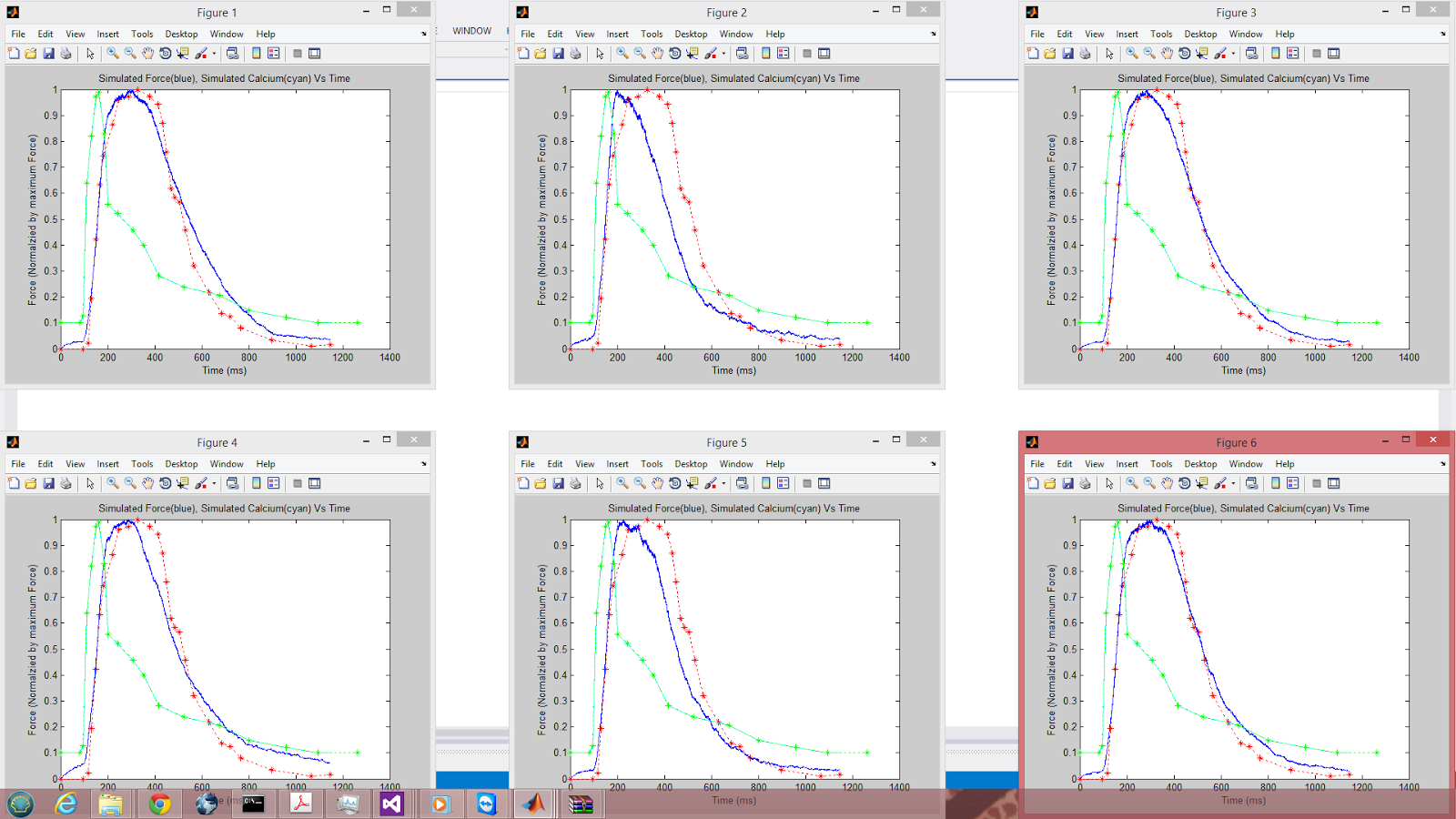
Allowing a calcium gradient means the transition matrix changes every time step in response to the calcium gradient. The solution was to compress the transition matrix to 51 unique values where a secondary "pointer matrix" mapped the original indices to an index in this unique-value array. Due to the compressed transition matrix, updating the matrix in response to calcium change is now a matter of updating these 53 unique values. Significantly speeds up the simulation. Code snippet below:
Such a model is highly appropriate to use with this framework due to its highly parallel structure and dependence on high quality random numbers being generated as quickly as possible. This is a feature shared by many biophysical simulations and is an area in computing that I consider to be the most benefitted from the framework I developed.
Results:
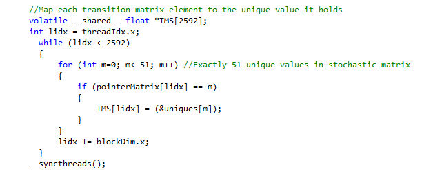
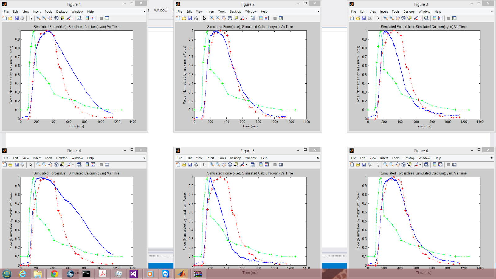
To demonstrate the power of my framework I will run through the results of optimizing my thin filament MCMC model. With my framework, I was able to fully utilize all my laptop's GPU's streaming multiprocessors (6 total) by running 6 particles in parallel. Using a serialized particle swarm or any other serialized optimization method would have been much less efficient as each kernel call only needs 1024 threads (reps). Rather than 17% occupancy, I get 100% occupancy and consequently, ~6x the performance.
Note that the model is attempting to fit the blue curve to the red curve (experimental muscle twitch) by modifying 12 physical parameters. The cyan curve represents a calcium gradient that was created by interpolating experimental calcium measurements from within the kernel. This curve should have the same values every iteration and is displayed for illustrative purposes.
Observe the convergence of the swarm for 6 parallel particles in just 300 PSO iterations:
Initial particles:
30% Complete
40% Complete
60% Complete
80% Complete
100% Complete
My framework converged to a global minimum. The particle swarm algorithm was clearly doing its job. Using the output file generated by my parallel PSO, we can see just how close all the particles are by comparing their positions across the same dimension:
Particle in swarm: 1, Iteration: 300, Cost: 2.983628e+02, Parameters:
[ 0.148912, 439.767975, 0.795025, 3.624428, 0.994157, 18.282904, 1.399269, ...
Particle in swarm: 2, Iteration: 300, Cost: 2.141252e+02, Parameters:
[ 0.148913, 439.851868, 0.795048, 3.593733, 0.994156, 18.064886, 1.398015, ...
Particle in swarm: 3, Iteration: 300, Cost: 2.892123e+02, Parameters:
[ 0.148911, 439.774323, 0.806439, 3.624597, 0.993891, 18.520998, 1.411488, ...
Particle in swarm: 4, Iteration: 300, Cost: 2.608216e+02, Parameters:
[ 0.148729, 439.743317, 0.795738, 3.623157, 0.999009, 18.279631, 1.399079, ...
Particle in swarm: 5, Iteration: 300, Cost: 2.385364e+02, Parameters:
[ 0.148912, 439.769867, 0.795027, 3.624206, 0.994173, 18.284321, 1.399272, ...
Particle in swarm: 6, Iteration: 300, Cost: 2.645783e+02, Parameters:
[ 0.148912, 439.767975, 0.795025, 3.624428, 0.994157, 18.282907, 1.399269, ...
Now, in order to check if the mex framework was doing it's job of parallelizing the model efficiently, I went to the Nvidia Visual profiler.
Current Nvidia GPU technology allows up to 32 particles to be run in parallel. I verify that my framework was capable of this parallelism by running my mex file as a standalone CUDA/C program on a Tesla k40c GPU after recompiling my mex file to take advantage of this architecture's hyper Q technology:
We can see that my framework is working as intended and has 32 streams running in parallel.
Next, to visualize a key paradigm of the GPU programming model, I used my framework to find the average run time per particle as a function of batch size on the Tesla k40c (15 SMs):
As expected, there are two minima in the curve, each trough at a multiple of 15, signifying equal workload across all SMs. This shows that, whenever possible, the total number of blocks being run in parallel should be a multiple of the number of SMs on the GPU.
But of course, this is a well established idea and does not offer specific insight on how to optimize my MCMC model. Therefore, I tested average run time per particle (n = 15) as a function of block size while keeping the total number of threads fixes at 1024:
These results are very interesting. Observe that taking 2 blocks instead of 1 reduces the average time by more than a factor of 2. This lopsided gain in efficiency means that the model can be run more efficiently when being run in blocks of two. The reason for this is that the kernel can more efficiently arrange its local variables to registers/caches when there are fewer threads being evaluated on an SM.
Using this information, I could optimize the launch bounds of my kernel so that instead having batches run:
1024 threads, 1 block => 15 seconds per batch => 1s /particle
I could run instead run:
512 threads, 2 blocks => 2 * 4.9 = 9.8 seconds per batch => 0.653s / particle!!!
It is clear that my framework enables users to optimize the launch bounds of their model.
Another feature it has that is a consequence of it's visualization capabilities, is the ability to test the minimum acceptable resolution of your stochastic model to allow faster optimization times due to less repetitions. I go through this process below:
1 repetition using the global best from a parallel PSO optimization
16 repetitions
128 repetitions
512 repetitions
Just for fun, 8192 repetitions
It would appear that using 512 repetitions would be a lower bound of acceptable resolution for my model for purposes of optimization. If I were having difficulty finding a good minimum, I would consider dropping the repetition count to 512 instead of the current 1024 in order to speed up the search.
In conclusion, this framework is a must-have if you are using PSO with a CUDA kernel. The framework not only offers enticing visualizations, but easy profiling of kernels and fast/efficient optimization on the GPU.
I expect to enhance the model to use more advanced PSO variants in the future, perhaps a genetic algorithm (GA). Depending on the popularity of this framework, I would also consider releasing a parallel version for CPU models that allow more control/customizability in multi-threading than what the Matlab parallel computing toolbox allows.
References:
(1) Eberhart, R., Shi, Y.: Comparing inertia weights and constriction factors in particle swarm optimization. In: Proceedings of the 2000 IEEE Congress on Evolutionary Computation, Piscataway, NJ, IEEE Press (2000) 84–88
Link to paper
(2) Campbell S. G., Lionetti F. V., Campbell K. S., Mcculloch A. D. 2010 Coupling of adjacent tropomyosins enhances cross-bridge-mediated cooperative activation in a Markov model of the cardiac thin filament. Biophys. J. 98, 2254–2264.
Link to paper